
Acoustic Basics - Basics of ultrasound wave composition
Understanding the Basics of US Wave Composition
In order to comprehend the upcoming acoustic concepts, we have to start with the fundamental building blocks of US:
1. Sound Wave
2. Wavelength and Frequency
In order to comprehend the upcoming acoustic concepts, we have to start with the fundamental building blocks of US:
1. Sound Wave
2. Wavelength and Frequency
1. Sound Wave
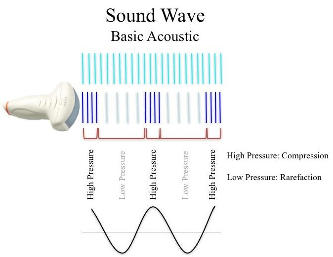
Here we have a diagram of a sound wave. On the top column in the babyblue, each line represents a group of particles in the air that are uniformly space and not moving. When an activated ultrasound probe is placed adjacent to this air column, it emits pulses of pressure waves. These waves cause compression of the particles in the air.
There are areas of high pressure where the particles are condensed followed by low pressure where the density of the particles is lower. Subsequently, these regions of high density, compression, and low density, rarefaction, alternate. This uniform pattern can be expressed as a Sine Wave.
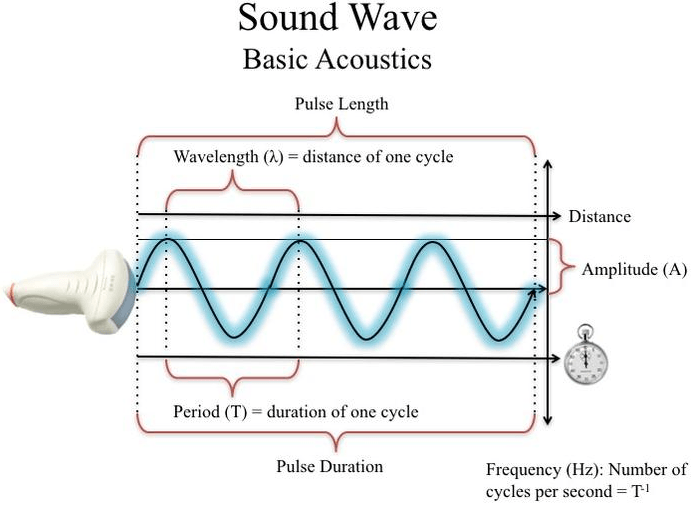
The ultrasound probe emits pulses of ultrasound waves
sequentially in a regular rhythmic fashion; and each pulse is composed of "n" number of cycles
with varying properties. What are these properties?
X-axis:
X-axis:
- Wavelength (λ): length of one cycle which is defined by the distance between two peaks or two troughs
- Period: duration of each cycle
- Frequency (Hz): inverse of period which in the number of cycles per second
- Amplitude: height of the wave - so-called intensity/strength of the wave
2. Wavelength and Frequency
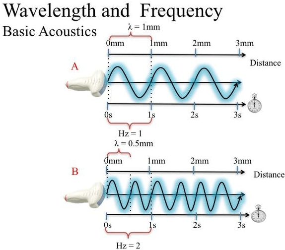
Let's focus on the relationship between λ and Hz for a bit more with the diagram. Here are two US pulses with one cycle demarcated for you in the red brackets.
Let's look at pulse A first. It has 3 cycles are present with each cycle characterized by λ = 1mm & Hz = 1. How about pulse B? It clearly has more cycles for the same given distance and time. The λ =0.5mm, half of pulse A's, and the Hz = 2, two cycles per second.
The main message of the diagram is to illustrate:
- as pulse's λ decreases, the Hz increases
- as pulse's λ increases, the Hz decreases
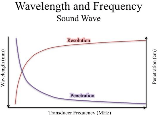
What is the practical imaging implication of λ and Hz? This diagram illustrates how the relationships between λ and Hz affect image resolution and penetration (how deep can the pulse US travel).
Key Points:
You cannot change the λ directly on the US machine. You can, however, select the frequency that you would like to employ. So, in this graph, the variable that you can control is the transducer frequency in the X-axis.
Key Points:
- The lower the MHz, the higher deeper the pulse US penetrates, but sacrificing resolution
- The higher the MHz, the higher the resolution, but at the cost of penetration
- Resolution and Penetration curves are NOT linear
You cannot change the λ directly on the US machine. You can, however, select the frequency that you would like to employ. So, in this graph, the variable that you can control is the transducer frequency in the X-axis.
Take Home Messages:
- Probe emits ultrasound PULSE consisting of “n” cycles
- Each cycle has a certain wavelength and frequency
- Wavelength is inversely related to frequency - a variable that can be controlled on the US machine
- The lower the pulse's frequency, the higher deeper the pulse US penetrates, but sacrificing resolution
- The higher the pulse's frequency, the higher the resolution, but at the cost of penetration